
Welcome and Happy New Year. I made a small tweak to the model, rearranging the layout of some of the initial settings, and to derive inertia from installed synchronous capacity rather than synchronous supply. An updated copy of the spreadsheet is available here (version 1.2).
Please remember, the model’s purpose is to help understand the transient response of power network. It’s not an exact model for a number of reasons – and some of the reasons I’ll expand on as I describe the variables and equations.
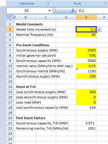
Here is the portion of the worksheet we are looking at with this post.
Model Constants
Model time increment [E3]: The time interval over which we calculate each step. I have set this to 0.1 second. Using the cell drop down you can also select either 0.05 or 0.2 second. Changing the step size affects model resolution and the overall time duration modelled.
Nominal Frequency [E4]: System nominal frequency. It is adjustable but I recommend leaving it at 50 Hz. I have fixed the scales of the primary and secondary axes of the graph to make use of common horizontal lines. Further, the 47 Hz minimum and 52 Hz maximum align with the frequencies where cascade tripping (blackout) is likely to occur. The red line (frequency) has to stay within the window.
Pre Event Conditions
Synchronous supply (MW) [E7]: This the combined output of all of the synchronous generators on the network. It isn’t their capacity or rating; it is their MW output just before the disturbing event.
The net power being injected into the network is the sum total of the Synchronous supply (MW) [E7] and Asynchronous supply (MW) [E12]. As mentioned above I have fixed the scales on the graph. The power scale is set to 2000 MW to 4000 MW, so to see what is going on, keep the total output toward the middle of that range. The network is presumed balanced (stable) pre-event, therefore net generation equals net connected load (plus grid losses).
Initial governor set point (%) [E8]: This setting defines the pre-event ‘average’ operating point of the synchronous machines.
Why ‘average’? A simplification made is that the synchronous machines on the grid are rolled up into one large machine with a single set of control characteristics. The real system (of course) has many machines operating, each with its own governor. Whilst the governors should have similar droop characteristics, they will be at various set points, and each should take account of the different response capability expected of its controlled machine. The Initial governor set point in the model represents an ‘average’ of all the operating synchronous machines on the grid. It is related to the spinning reserve. The MW difference between the set point in terms of MW, and the total of the synchronous machine capacities’, is ‘spinning reserve’.
Synchronous capacity (MW) [E9]: This is the pre-event net total of the output power ratings of all the synchronously connected generators. It is derived from the above two factors: E9=E7/E8.
Inertial ratio (MWs/Hz to MW capacity) [E10]: This is the available rotational kinetic energy in megawatt seconds, per Hertz of speed change, per megawatt of synchronous machine rating.
Another simplification made is the relationship between kinetic energy and speed. Kinetic energy of a rotating mass is proportional to the square of rotational speed, and therefore dependent on frequency. However as we’re interested in speed (frequency) changes near to 50 Hz, (within 2 or 3 Hz) we don’t lose much accuracy by taking the kinetic energy as proportional to frequency (i.e.: linear for that small range / a constant inertial ratio).
Synchronous inertia (MWs/Hz) [E11]: This is the pre-event net total inertia. It is derived from the above two factors: E11=E9*E10.
Asynchronous supply (MW) [E12]: This is the combined megawatt output from all of the asynchronous generators on the network. This would generally be the combined output of all the wind and solar generation at the time of the event.
It may not be, but given the short duration modelled, this generation is taken as constant through the event period (unless we have chosen it as the loss event, or unless we have chosen to turn on IBFFR, Inertia Base Fast Frequency Response. There’ll be more on IBFFR in a later post).
Event at T=0
Three types of event are allowed. Choose the event by entering the MW disturbance in the appropriate cell.
Lose synchronous supply (MW) [E15]: Entering a number of MW in this cell represents loss of synchronous generation, at its pre event operating level. (i.e.: not the MW generator capacity). Losing synchronously generated MW affects both remaining inertia and available generation.
Lose asynchronous supply (MW) [E16]: Entering a number of MW in this cell represents loss of asynchronous generation, at its pre event operating level. (i.e.: not the generator MW capacity). Whilst losing asynchronous generation does reduce available generation, it does not reduce remaining inertia (because it offered none in the first place).
Lose load (MW) [E17]: The third type of event that can be simulated is a loss of load, i.e.: maybe the loss of a major feed into a city or a region. This should be a rare type of event (often referred to as non-credible) given that the network at this level should have built-in redundancy and it would take a double failure for it to occur. A loss of load event results in a frequency rise rather than a decline, generation input exceeds demand and the generators speed up.
Lost synchronous capacity (MW) [E18]: With the loss of synchronous supply also comes loss of synchronous capacity, and this is estimated in this model to be in proportion to the lost supply and inverse of the initial governor set point. It is derived from these two factors where E18=E15/E8.
Post Event Factors
Synchronous capacity, T>0 (MW) [E21]: This field calculates the remaining synchronous capacity after the disturbing event by deducting the lost synchronous capacity from that prior to the event, i.e.: E21=E9-E18.
Remaining inertia, T>0 (MWs/Hz) [E22]: This field calculates the remaining synchronous inertia after the disturbing event from the remaining synchronous capacity and inertial ratio, i.e.: E22=E21*E10.
That’s enough for now. The next post will focus on governor characteristics.
Anthony
One possible issue with your model is the governor droop function. Much of the generation on the grid at any one time is at or near full load. This is all the geothermal, often the thermal as well and much of the hydro. That means that they can offer no support in under-frequency events as they are already at 100%. For even partially loaded generators, they can only support to the limits of their headspace between actual generation and rating. The total generation available to ramp up is less than 500MW – from the look of the generation data, typically 2-300MW at a guess.
To get around this, you would only need an additional box giving available generation. The effect of this limitation is significantly lowering the response. It also allows the value of partly loaded machines to be easily demonstrated. For significant overfrequency (like power going south and the DC tripping), the grid operators are using a station trip at Te Mihi, rather than just governors backing the load off.
To add to governor response, there is the misunderstood spinning reserve. Tokaanu and a couple of the SI units used to have tailrace depression to allow synchronous spinning reserve. I don’t know if the grid operators still use that function or even it is still working. From the recent big underfrequency events, it doesn’t look like they do. Rather, it is load shedding and bringing up partially loaded hydros like Maraetai quickly in a dispatch, rather than governor function. I am not sure of that though, as the Historian data discrimination is coarse.
Thanks for the comments Chris.
Yup, a large proportion of synchronous generation runs in the 90% to 100% range and therefore upward droop response from those machines is very limited. However, this can be represented (in an overall average way) in the model.
Refer to cells E7, E8 and E9. The example shows 3500 MW of generation output, a 70% governor setting, and a calculated machine capacity of 5000 MW. (5000 = 3500 / 0.7). This would be a pre event ‘headspace’ of 1500 MW.
To accommodate a lower level of ‘headspace’, simply set the governor setting, cell E8, to a higher value. The spreadsheet derives two available capacities. The pre event synchronous capacity is in cell E9. The post event capacity is in cell E21.
Your point about modelling two sorts of synchronous generator rather than a single ‘average’ machine would be interesting. Maybe it could be a future development. Thanks for the thought.
Question for you: I’ve always taken what you’ve referred to as ‘head space’ and spinning reserve as effectively the same thing. i.e.: already synchronised generation that is available to be ramped up, either under governor control or at the request of the system operator. But I note you refer to them separately. Could you expand on your interpretation?
Anthony
I always referred to spinning reserve as machines available to generate, linked into the grid as synchronous condensers, but not actually generating. This would be plant like Tokaanu on tailrace depression and the wicket gates shut. From a plant operator’s point of view, they are on grid support (ancillary services), but would have no generation income.
The headspace is for partially loaded generating machines, but only if they are on governor, not load limiter or high droop control. (For the latter, from memory, the thermal plant used to have two governor settings; 4% droop and 25% droop). Load limiters allow the governing valves to shut on governor control, but not to open. Essential on part loaded geothermal plant to stop water carryover into the pipelines during an underfrequency.
You are correct in your assumption that they effectively do the same thing.
You are doubtless correct where the NZ grid is concerned, but these posts have a wider audience, so I think it a good idea to allow a wider range of operating conditions to be simulated, rather than aiming exclusively at reproducing NZ circumstances.
I think the real strength of providing these models is to offer something that can be tweaked to give at least a first order idea of what can happen in e.g. King Island, Tasmania, or South Australia (equally, Ireland so far as wind is concerned) with its heavy wind and solar dependence, etc.
Politicians around the world are making bad decisions for the future because they don’t understand these concepts, or their importance in keeping the lights on. I think it’s really good to have something simple that can show them what might happen if they went ahead with their bonkers ideas, and the limitations of some of the solutions that they are being encouraged to rely upon.
Thanks you for your comments. All valid points. And I can see that Chris has replied below too. Thanks to you too Chris.
It doesn’t add up, your last paragraph describes very well why I’m doing this series on power system stability. The intention is for more folk to understand this, especially to help them understand and to explain the folly of zero inertia and no governor control. While my present example is related to a North Island (NZ) event, I do expect the model to usefully show ‘first order’ effects as you describe. I want to work through the model piece by piece explaining in some details what these factors are, so that others can adjust and observe.
I’m pleased that you and Chris are following along. As we work on this I do expect that other features could be added. Please do understand though, this is still a work in progress and very much a spare time activity for me so it will take me a fair while sometimes between posts and replying to comments.
I have not tried to use your model. However, it is not evident to me that you have made any allowance for stored energy (kinetic energy) in the load.
You’re right Richard, good observation.
Indeed, I have not attempted to model any kinetic energy in the load. There would potentially be two kinetic energy effects to consider, inertia and power draw.
The inertial effect is small due to low coupling between the rotational kinetic energy and the magnetic field linking to the power system. While there certainly is kinetic energy in the load (mainly rotational load on induction machines) because it is not synchronously connected it provides next to no inertial response. Also most larger machines now are controlled by electronics. This completely decouples the kinetic energy from the network. This even applies to smaller home appliances like washing machines, food mixers etc. All are controlled by electronics.
In regard to power draw as the frequency falls, there would be some effect. However, this is limited to only those smaller induction motors directly connected to the system. These are becoming fewer as electronic controls are being applied to almost every appliance.
It doesn’t add up.
Anthony will correct me if I am wrong, but NZ is a very good example to use to build and calibrate a model. This is because the largest generator is about 8% of the grid, so trips give a significant frequency fluctuation that shows real governor response. See his previous worked examples. It also has all the generation types (except pumped storage) running different operational modes, few significant transmission constraints, a DC interconnector that can and does go both ways for grid management, and very active demand management by some of the large industrial users, the biggest of which is bigger than the largest generator. The generation and frequency data is also readily available. Once he can show it works for NZ, then it could be tweaked to work elsewhere.
From my reading of the AEMO report, this model would be of little use to analyse the SA blackout. That was caused by; wrong protection settings on the wind turbine stations, overloading of the line in from Victoria tripping it, and then too rapid RoCoF to allow block load shedding. By the time the got to the last point, it was already gone.
Thanks Chris, your reply is more generous than what I actually thought. I have simply calibrated the model with the Stratford trip on 15/06/17 example because that was the event that I had all the necessary data for. And some of that data was from you, which you provided in the discussions in the earlier series of posts. So thank you for your continued interest as we put this thing together.
Anthony
For the NZ system with a lot of hydros on, isn’t there a kinetic/ inertia effect on underfrequency from the water in the penstocks having to accelerate as the wicket gates open? There are similar problems on boiler plant with the lag between increased burn rate and more steam being available. I’m not certain how the governor response curves deal with that.
I should have explained deeper for other readers about my last comment. The standard industry method for proving governor response to variable load (droop) is by opening the circuitbreaker when the machine is at part load. The speed rise can then give you both response rate and time.
However, in a real life situation on a hydro or boiler plant, there is a real lag between the governor opening the valves/ gates and the fluid being there to generate the power. This can be an important factor to consider in even a simple model. System Operator may cover this by their fast and slow response reserve data.
The generation data shows that Tiwai is now giving a lot of grid support – There are numerous irregular drops in load of about 150 MW. They seem to coincide with other events, so I surmise that they are providing the fast reserve, rather than having to use hydros with tailrace depression.
Sorry, the above post is from me, not a different commenter.