Modelling Power System Stability – Part 2, System Variables and Conditions

Welcome and Happy New Year.  I made a small tweak to the model, rearranging the layout of some of the initial settings, and to derive inertia from installed synchronous capacity rather than synchronous supply.  An updated copy of the spreadsheet is available here (version 1.2).

Please remember, the model’s purpose is to help understand the transient response of power network.  It’s not an exact model for a number of reasons – and some of the reasons I’ll expand on as I describe the variables and equations.

Here is the portion of the worksheet we are looking at with this post.
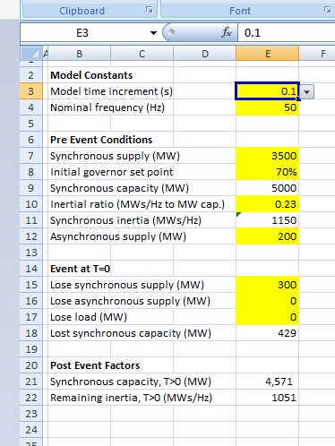
Model Constants

Model time increment [E3]: The time interval over which we calculate each step.  I have set this to 0.1 second.  Using the cell drop down you can also select either 0.05 or 0.2 second.  Changing the step size affects model resolution and the overall time duration modelled.

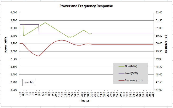
Nominal Frequency [E4]:  System nominal frequency.  It is adjustable but I recommend leaving it at 50 Hz.  I have fixed the scales of the primary and secondary axes of the graph to make use of common horizontal lines.  Further, the 47 Hz minimum and 52 Hz maximum align with the frequencies where cascade tripping (blackout) is likely to occur.  The red line (frequency) has to stay within the window.

Pre Event Conditions

Synchronous supply (MW) [E7]: This the combined output of all of the synchronous generators on the network.  It isn’t their capacity or rating; it is their MW output just before the disturbing event.

The net power being injected into the network is the sum total of the Synchronous supply (MW) [E7] and Asynchronous supply (MW) [E12].  As mentioned above I have fixed the scales on the graph.  The power scale is set to 2000 MW to 4000 MW, so to see what is going on, keep the total output toward the middle of that range.  The network is presumed balanced (stable) pre-event, therefore net generation equals net connected load (plus grid losses).

Initial governor set point (%) [E8]:  This setting defines the pre-event ‘average’ operating point of the synchronous machines.

Why ‘average’?  A simplification made is that the synchronous machines on the grid are rolled up into one large machine with a single set of control characteristics.  The real system (of course) has many machines operating, each with its own governor.  Whilst the governors should have similar droop characteristics, they will be at various set points, and each should take account of the different response capability expected of its controlled machine.  The Initial governor set point in the model represents an ‘average’ of all the operating synchronous machines on the grid.  It is related to the spinning reserve.  The MW difference between the set point in terms of MW, and the total of the synchronous machine capacities’, is ‘spinning reserve’.

Synchronous capacity (MW) [E9]:  This is the pre-event net total of the output power ratings of all the synchronously connected generators.  It is derived from the above two factors:  E9=E7/E8.

Inertial ratio (MWs/Hz to MW capacity) [E10]:  This is the available rotational kinetic energy in megawatt seconds, per Hertz of speed change, per megawatt of synchronous machine rating.

Another simplification made is the relationship between kinetic energy and speed.  Kinetic energy of a rotating mass is proportional to the square of rotational speed, and therefore dependent on frequency.  However as we’re interested in speed (frequency) changes near to 50 Hz, (within 2 or 3 Hz) we don’t lose much accuracy by taking the kinetic energy as proportional to frequency (i.e.: linear for that small range / a constant inertial ratio).

Synchronous inertia (MWs/Hz) [E11]:  This is the pre-event net total inertia.  It is derived from the above two factors:  E11=E9*E10.

Asynchronous supply (MW) [E12]:  This is the combined megawatt output from all of the asynchronous generators on the network.  This would generally be the combined output of all the wind and solar generation at the time of the event.

It may not be, but given the short duration modelled, this generation is taken as constant through the event period (unless we have chosen it as the loss event, or unless we have chosen to turn on IBFFR, Inertia Base Fast Frequency Response. There’ll be more on IBFFR in a later post).

Event at T=0

Three  types of event are allowed.  Choose the event by entering the MW disturbance in the appropriate cell.

Lose synchronous supply (MW) [E15]:  Entering a number of MW in this cell represents loss of synchronous generation, at its pre event operating level.  (i.e.: not the MW generator capacity).  Losing synchronously generated MW affects both remaining inertia and available generation.

Lose asynchronous supply (MW) [E16]:  Entering a number of MW in this cell represents loss of asynchronous generation, at its pre event operating level.  (i.e.: not the generator MW capacity).  Whilst losing asynchronous generation does reduce available generation, it does not reduce remaining inertia (because it offered none in the first place).

Lose load (MW) [E17]:  The third type of event that can be simulated is a loss of load, i.e.: maybe the loss of a major feed into a city or a region.  This should be a rare type of event (often referred to as non-credible) given that the network at this level should have built-in redundancy and it would take a double failure for it to occur.  A loss of load event results in a frequency rise rather than a decline, generation input exceeds demand and the generators speed up.

Lost synchronous capacity (MW) [E18]:  With the loss of synchronous supply also comes loss of synchronous capacity, and this is estimated in this model to be in proportion to the lost supply and inverse of the initial governor set point.  It is derived from these two factors where E18=E15/E8.

Post Event Factors

Synchronous capacity, T>0 (MW) [E21]:  This field calculates the remaining synchronous capacity after the disturbing event by deducting the lost synchronous capacity from that prior to the event, i.e.:  E21=E9-E18.

Remaining inertia, T>0 (MWs/Hz) [E22]:  This field calculates the remaining synchronous inertia after the disturbing event from the remaining synchronous capacity and inertial ratio, i.e.:  E22=E21*E10.

That’s enough for now.  The next post will focus on governor characteristics.

Posted in Power System Stability | 13 Comments

Modelling Power System Stability – Part 1

In a comment Stuart asked “Any chance of a post on synthetic inertia from PV/wind turbines/HVDC links, and why it does or doesn’t help? I keep reading that curtailing the output from the maximum to give some ‘headroom’ allows these things to react similarly and replace rotating generators with electronics, helping stability.”

Well Stuart, great comment – here goes.  There are two main themes you’ve included in your comment, curtailment and synthetic inertia.

In order to tackle this I developed a power system stability model.  It’s an Excel spreadsheet using a stepwise (0.1 second) time domain development of the swing equation df/dt = P/M and some generation and load response mechanisms/characteristics.

A copy of the Excel worksheet is available here.  Please do download a copy.

Before we look at the questions I’d like to explain how the model works, the equations used and some of the limitations.  It’ll take a few posts and a degree of patience, so if you’re interested please follow along. And feel free to ask a question.

The sheet is not locked in any way so be careful how and where you type.  However, if you do happen to mess it up, you can always come back and download a fresh copy.

Here’s a quick overview of the sheet.  Input variables are shaded yellow (which should be the only cells you need to modify).

The blocks of input data requirements are; the pre event conditions, the disturbing event at time T=0, the governor characteristics, the battery based response, the under frequency load shedding, the rate of change load shedding, and the inertia based fast frequency response.  Each one of these will be discussed in more detail in later posts.

The calculation table from Row 27 down steps through the simulation one model increment at a time.  Each line calculates the power imbalance, which acts upon system inertia to produce a frequency change.  The resulting frequency and rate of change of frequency is applied to the system control elements to produce the power conditions for the next increment.  These equations too will be described in future posts.

The graph below is an example of the output from the model.  It shows net generation in green, net load in purple, and system frequency in red.  Here’s what happens in this example:

The system is running stably with 3500 MW of synchronous generation and 200 MW of asynchronous generation, net generation 3700 MW.  At time T=0 the system loses 300 MW of synchronous generation, net generation drops to 3400 MW, and the frequency starts to fall because the net load is still 3700 MW.

The synchronous governors sense the frequency dropping and begin increasing output.  The rate of frequency decline is reducing as generation increases.  At the point when the frequency hits 49.2 Hz (4.8 seconds) the first block of under frequency shedding occurs.  The load drops by 222 MW to 3478 MW.  At this time the generation is at 3647 MW and so the frequency commences recovery.

The governor continues to sense both frequency and rate of change of frequency and adjusts output using droop, differential and machine limits to restore power balance at a slightly lower frequency after around 20 seconds.

Posted in Power System Stability | 4 Comments

Cosmics Leaving Outdoor Droplets – CLOUD

About six years ago I posted an article about CLOUD, an experiment to better understand the correlation between intensity of cosmic rays which varies with the sunspot cycle (solar activity), and cloud formation.  In summary the findings to date indicate that the effect of cosmic rays on cloud formation is small compared to the large variations in natural biogenic aerosol emissions.

A paper by Hamish Gordon, Jasper Kirkby and thirty others titled “Causes and importance of new particle formation in the present-day and pre-industrial atmospheres”.

[doi: 10.1002/2017JD026844]

The abstract states: [my bold]

New particle formation has been estimated to produce around half of cloud-forming particles in the present-day atmosphere, via gas-to-particle conversion.  Here we assess the importance of new particle formation (NPF) for both present-day and pre-industrial atmospheres. …

Concerning causes, we find that the importance of biogenic volatile organic compounds (BVOCs) in NPF and CCN formation is greater than previously thought. …

Our model suggests that the effect of changes in cosmic ray intensity on CCN is small and unlikely to be comparable to the large variations in natural primary aerosol emissions.

Posted in Climate Science | 2 Comments

7. Analysis of an under frequency event

Let’s take a closer look at the under frequency event that occurred at 9.51am on Thursday June 15th 2017, in the North Island of New Zealand. This is quite a long post with quite a bit of technical detail.

The event was caused by the loss of generation at a gas fired power station in Stratford, Taranaki. Chris (chrism56) advised in comments on the previous post that it was the TCC (Taranaki Combined Cycle) power station that tripped, and that it was generating 310 MW just before it tripped. He checked some other generator outputs at that time and as he didn’t observe any significant droop pick up on the ones he looked at he deduced automatic under frequency shedding most likely operated. Good work Chris, turns out you were right.

There are a number of industrial plants contracted to immediately disconnect selected loads if the frequency falls to 49.2 Hz.

The graph below which is based on 5 minute load data from NZ’s System Operator confirms that load shedding occurred. The North Island load can be seen to drop 300 MW, from 3700 MW at 9.50 to 3400 MW at 9.55. The load restoration phase can also be observed from this graph. From 10.15 through 10.40 the shed load is restored in several steps.

The high resolution data that we’ll be looking at more closely was recorded by a meter with power quality and transient disturbance recording capability. It is situated in Masterton, Wairarapa, about 300 km south of the power station that tripped. The meter is triggered to capture frequency excursions below 49.2 Hz. The graph below shows the captured excursion on June 15th. The graph covers a total period of only one minute. It shows the frequency and Masterton substation’s load. I have highlighted and numbered several parts of the frequency curve to help with the discussion.

The analysis makes use of the equation P = M * df/dt, which is very similar to the equation developed in an earlier post. Here P is the grid net power imbalance in MW, M is the grid angular momentum in MWs/Hz, and df/dt is the rate of change of frequency in Hz/s.

The first element we’ll look at is element 1 to 2. The grid has just lost 310 MW generation and the frequency is falling. No governors nor load shedding will have responded yet. The frequency falls 0.192 Hz in 0.651 seconds giving a fall rate df/dt of -0.295 Hz/s. From this df/dt result and knowing the lost generation is 310 MW we can derive the system angular momentum M as 1,052 MWs/Hz from -310 = M * -0.295.

It is interesting (and chilling) to calculate how long it would take for blackout to occur if no corrective action is taken to restore system frequency and power balance. 47 Hz is the point where cascade tripping is expected. Most generators cannot operate safely below 47 Hz, and under frequency protection relays disconnect generators to protect them from damage. This sets 47 Hz as the point at which cascade outage and complete grid blackout is likely. A falling frequency of -0.295 Hz/s would only take 10.2 seconds to drop from 50 to 47 Hz. That’s not very long and obviously automated systems are required to arrest the decline. The two common automatic systems that have been in place for decades are governor controlled generators and various levels of load shedding.

The next two elements we’ll look at are 3 to 4 and 5 to 6. From 3 to 4 the df/dt fall rate is -0.108 Hz/s. Using this df/dt and M for the system derived above,1,052 MWs/Hz, the imbalance is now a deficit of 114 MW. From 5 to 6 the frequency in increasing and df/dt is 0.095Hz/s. Using this df/dt and M as before, the imbalance is now a surplus 100 MW. The fall arrest between 4 and 5 has been due to automatic load shedding. New Zealand has a number of customers contracted to disconnect load at 49.2 Hz. From these figures we can estimate a net shed load of 214 MW (114 MW + 100 MW). The sudden drop in Masterton substation’s load from about 36.4 MW to 35.6 MW occurs as the frequency passes down through 49.2 Hz, (point 4 in the graph). It indicates that about 0.8 MW of the 214 MW was from Masterton substation’s load.

From 7 to 8 the frequency is increasing with df/dt of 0.111 Hz/s and the system has a surplus of 117 MW of generation. At point 8 the system reached 50 Hz again, but the system then over shoots a little and governor action works to reduce generation to control the overshoot between 8 and 9.

Another interesting event takes place between 10 and 11. It seems there is another (too late to be useful) load shed event. From 9 to 10 df/dt is -.039 Hz/s and a deficit of 41 MW. From 11 to 12 df/dt is 0.031 Hz/s and a surplus of 33 MW. This indicates a further 74 MW is shed in the period 10 to 11. It becomes necessary that the governors again sense the increasing frequency and pull it back after it moves up through 50.2 Hz.

This analysis shows how system inertia, under frequency load shedding and governor action work together to maintain system stability.

The analysis derived a total of 288 MW shed load (214 MW + 74 MW). As this was based on a differential analysis of system frequency it would not be an exact analysis. However, the result of 288 MW is close to the 300 MW drop shown on the North Island Load graph shown at the start of this post.

The table below provides a summary of the calculated results for the selected graph elements.

The data and graph may be found in a spreadsheet here:

The key points:

  • The system needs to be able to maintain stability second by second, every minute, every hour, every day, year after year.  Yet when a major disturbance happens, the time available to respond is only a few seconds.

  • This highlights the essential role of system inertia in providing this precious few seconds. System inertia defines the relationship between power imbalance and frequency fall rate. The less inertia the faster the collapse and the less time we have to respond.  Nearly all system inertia is provided by synchronous generators.

  • Control of the input power to the generators by governor action is essential to control frequency and power balance, bringing correction to maintain stability. This requires control of prime mover, typically this is only hydro and thermal stations.

  • When the fall rate is too fast for governor response, automatic load shedding can provide a lump of very helpful correction, which the governors later tidy up by fine tuning the response.

Index

  1. Introduction – Electric Power System Stability
  2. Electric current is generated ‘on demand’. There is no stored electric current in the grid
  3. Energy balance, imbalance and a definition of grid stability
  4. Generator types; synchronous versus asynchronous. What goes on inside the machines?
  5. Frequency stability and energy balance. A description of the interaction between frequency and grid energy flow
  6. Control of the prime mover, governors, how it is done and why it matters
  7. Analysis of an under frequency event
Posted in Electricity, Power System Stability | 14 Comments

6. Control of the prime mover, governors, how it is done and why it matters

The previous article described the relationship between power imbalance and rate of frequency change for the first few seconds after a disturbance in power balance. Important as those few seconds are, the few seconds of energy being provided by the spinning angular momentum of the synchronous machines, if something isn’t done to correct the power imbalance within those few seconds, collapse will certainly follow in only a few more seconds. Feedback control is the key to this response. The machine governor is the all important device providing the control … and if there is insufficient governor response the backstop is load shedding triggered by under frequency relays.

The diagram below shows how a governor fits in the system as a feedback controller. The governor’s purpose is to sense the shaft rotational speed, and the rate of speed increase /decrease, and to adjust machine input via a gate control.

Remember that shaft rotational speed w is directly aligned with frequency, and that frequency has to be kept within about +/- 0.5 Hz of nominal, and that power imbalance, angular momentum and rate of frequency change is described by Pm – Pe = M * dw/dt.

Starting with an initial condition where the machine running a constant speed w, Pm = Pe and dw/dt =0. When more electrical load Pe is taken from the generator (Pe>Pm), rotational energy will be extracted from the machine and it will slow (dw/dt<0).  Of course the opposite would happen if less electrical load was taken from the generator.

The governor’s job is to continuously monitor the rotational speed w of the shaft and the rate of change of shaft speed dw/dt and to control the gate(s) to the prime mover. In the example below, a hydro turbine, the control applied is to adjust the flow of water into the turbine, and increasing or reducing the the mechanical power Pm compensate for the increase or reduction in electrical load,  ie: to approach equilibrium.

It should be pointed out that while the control systems aim for equilibrium, true equilibrium is never actually achieved. Disturbances are always happening and they have to compensated for continuously, every second of every minute of every hour, 24 hours a day, 365 days a year, year after year.

The discussion has been for a single synchronous generator, whereas of course the grid has hundreds of generators. In order for each governor controlled generator to respond fairly and proportionately to a network power imbalance, governor control is implemented with what is called a ‘droop characteristic’. Without a droop characteristic, governor controlled generators would fight each other each trying to control the frequency to its own setting. A droop characteristic provides a controlled increase in generator output, in inverse proportion to a small drop in frequency. Refer to the graph below.

The governor senses system frequency and it controls it’s generator’s prime mover to increase the generator’s output according to the droop characteristic. The droop slope is typically referred to in percentage terms. It is typically about 4%. This equates to 2 Hz drop in a 50Hz system for a 0% to 100% change in generator output.

In New Zealand the normal operational frequency band is 49.8 to 50.2 Hz. An under frequency event is an event where the frequency drops to 49.25 Hz. It is the generators controlled by governors with a droop characteristic that pick up the load increase and thereby maintain stability.  If it happens that the event is large and the governor response is insufficient to arrest the falling frequency, under frequency load shedding relays turn off load.

Here is a record of an under frequency event earlier this month, where a power station tripped.

The generator tripped at point A which started the frequency drop. The rate of drop dw/dt is determined by size of the power imbalance divided by the synchronous angular momentum (Pm – Pe)/M. In only 6 seconds the frequency drop was arrested at point B by other governor controlled generators and under frequency load shedding, and in about 6 further seconds additional power is generated, once again under the control of governors, and the frequency was restored to normal at point C. The whole event lasting merely 12 seconds.

So why would we care about a mere 12 second dip in frequency of less than 1 Hz. The reason is that without governor action and under frequency load shedding, a mere 12 second dip would instead be a complete power blackout of the North Island of New Zealand.

The next article will look more closely at this event.

[Article updated 9 Jul 17 following comments from chrism56.  Thanks Chris]

Index

  1. Introduction – Electric Power System Stability
  2. Electric current is generated ‘on demand’. There is no stored electric current in the grid
  3. Energy balance, imbalance and a definition of grid stability
  4. Generator types; synchronous versus asynchronous. What goes on inside the machines?
  5. Frequency stability and energy balance. A description of the interaction between frequency and grid energy flow
  6. Control of the prime mover, governors, how it is done and why it matters
  7. Analysis of an under frequency event
Posted in Electricity, Power System Stability | 18 Comments

5. Frequency stability and energy balance. A description of the interaction between frequency and grid energy flow.

In an earlier post I gave a definition of a stable power system.

A stable power system is one that continuously responds and compensates for power/ frequency disturbances, and completes the required adjustments within an acceptable timeframe to adequately compensate for the power/frequency disturbances.

This post delves into the mathematics of what happens in the first few seconds after a disturbance. So apologies – this post does involve some maths.

The first few seconds after a power balance disturbance is analysed using Newton’s laws of motion. We’re going to look at the power flow between the rotating inertia (rotational kinetic energy) of a synchronous generator and the power system. It applies for the first few seconds after the onset of a disturbance, i.e.: before the governor and prime mover have had opportunity to adjust the input power to the generator.

We begin with the rotational form of Newton’s second law of motion; Force = Mass * Acceleration.

T = J * d2A/dt2

T is the net accelerating torque applied to the rotor. T is the difference between the driving torque of the prime mover Tm, and the retarding torque from the electrical load Te. i.e.: T = Tm – Te.

J is the moment of inertia of the rotor (and the attached prime mover)

A is the angle of the rotor with respect to a fixed reference

d2A/dt2, is the second differential of angular position with respect to time, the rotational acceleration of the of the rotor

We’ll define w as the rotational speed of the rotor, i.e.: dA/dt . w is equivalent to frequency.  The shaft acceleration d2A/dt2 is equivalent to the rate of change of rotor speed dw/dt. The shaft power is the product of torque and angular speed; i.e.: P = T * w, and angular momentum M is the product of moment of inertia and angular speed; i.e.: M = J * w. Using these we can derive the following equation:

Pm – Pe = M * dw/dt

Pm is the mechanical power being applied to the rotor by the prime mover. We consider this is a constant for the few seconds that we are considering.

Pe is the electrical power being taken from the machine. This is variable.

M is the angular momentum of the rotor and the directly connected prime mover. We can also consider M a constant, although strictly speaking it isn’t constant because it depends on w.  However as w is held within a small window, M does not vary more than a percent or so.

dw/dt is the rate of change of rotor speed, which relates directly to the rate of increasing or reducing frequency.

The machine is in equilibrium when Pm = Pe. This results in dw/dt being 0, which represents the rotor spinning at a constant speed. The frequency is constant.

When electrical load has been lost Pe is less than Pm and the machine will accelerate resulting in increasing frequency. Alternatively when electrical load is added Pe is greater than Pm the machine will slow down resulting in reducing frequency. Here’s the key point, for a given level of power imbalance the rate of rise and fall of system frequency is directly dependent on synchronously connected angular momentum, M.

It should now be clear how central a role that synchronously connected angular momentum plays in power system stability. It is the factor that determines how much time generator governors and automatic load shedding systems have to respond to the power flow variation and bring correction.

In the above I have made some simplifications. I have presumed a simple two pole machine, ignored machine losses and damping, and not talked about units used. This has simplified the equations and shortened the discussion, while keeping the important concepts in place. If readers do want to understand this in more detail there are good text books on the topic; but be warned, the mathematics gets very intense.

Power System Control and Stability, PM Anderson and AA Fouad, Wiley Interscience, IEEE Press.

Power System Stability and Control, Prabha Kundur, McGraw-Hill Inc.

Electric Power Systems, Analysis and Control, Fabio Saccomanno, Wiley Interscience, IEEE Press.

Next article – governor controls.

Index

  1. Introduction – Electric Power System Stability
  2. Electric current is generated ‘on demand’. There is no stored electric current in the grid
  3. Energy balance, imbalance and a definition of grid stability
  4. Generator types; synchronous versus asynchronous. What goes on inside the machines?
  5. Frequency stability and energy balance. A description of the interaction between frequency and grid energy flow
  6. Control of the prime mover, governors, how it is done and why it matters
  7. Analysis of an under frequency event
Posted in Electricity, Power System Stability | 2 Comments

4. Generator types; synchronous versus asynchronous. What goes on inside the machines?

There are two main types of alternating current machine used for the generation of electricity; synchronous and asynchronous.  The difference between them begins with the way the magnetic field of the rotor interacts with the stator.  Both types of machine can be used as either a generator or motor.

Synchronous Machine

Let’s start by describing a synchronous generator.  The rotor is basically just a magnet on a shaft.  In practice the magnet is generally an electromagnet.  The stator consists of three coils of wire placed to intersect with the rotor’s magnetic field, equally spaced around the circumference, 120o apart.  Each coil supplies current for one phase of the grid.  As the rotor rotates past each coil the induced current in each coil rises and falls in positive and negative directions as the north and south poles of the rotor passes by.  Each revolution generates one cycle of current.  The frequency generated is directly related to the speed of rotor revolution.  For a single magnet (two pole) machine, 50 Hz is generated when rotating at 3000 RPM.  A rotor with four poles generates 50 Hz when rotating at 1500 RPM.

Therefore the operating rotational speed of a synchronous machine is essentially a constant (within a small window).  Its speed is tied to system frequency.  Synchronous machines are governor controlled.  The governor monitors the system frequency and adjusts the machine’s prime mover power to bring correction to the frequency.  This is of course subject to the power capability of the machine and whether it is operating at power setting where increases (and reductions) can readily be made.

As mechanical power is applied to the shaft the rotor advances in relation to the rotating field generated by the system voltages on the stator coils.  The machine still remains in rotational synchronism with the system voltages, but the rotor is now in advance of the system by an angle d.  The angle d varies with the power being applied and generated, where the power is proportional to Sin(d).  If d is positive the machine is in advance of the system and is acting as a generator.  If d is negative the machine is being pulled along by the system, and it is acting as a motor.  If d is zero, the machine is spinning but no energy transfer is occurring.  Observe that Sin(d) maximises at 90o.  This is the rotor advance angle limit relating to the theoretical maximum torque that the machine is capable of delivering.

Here’s a mechanical analogy of a synchronous machine that might help.  Imagine the magnetic torque between the rotor and stator as being a spring connecting two rotating wheels.  The first wheel is connected to the driving source, ie: the rotor.  The second wheel represents the power system load.  As some extra loading is applied to the second wheel the angle between the wheels begins to increase as the spring stretches.  More torque is transferred via the stretched spring and kinetic energy moves from the directly connected spinning mass of the first wheel to the second.


Asynchronous Machine

As would be expected by the naming, the main difference between asynchronous and synchronous machines is about rotor synchronism.  The rotor of an asynchronous generator does not run synchronism with system voltages.   An asynchronous machine operates with ‘slip’.  ‘Slip’ is a percentage measure of how much slower or faster the rotor runs compared to its synchronous speed.  When the rotor is rotating slower than synchronous speed the machine acts as a motor. When the rotor is rotated faster than synchronous speed the machine acts as a generator.

Here’s a mechanical analogy of an asynchronous machine that might help.  Imagine the magnetic torque between the rotor and stator as being a hydraulic fluid coupling between two wheels.  The first wheel is connected to driving source, ie: the rotor.  The second wheel represents the power system.  As some extra loading is applied to the second wheel the hydraulic coupling slips more, but the flow of kinetic energy from the first wheel is largely decoupled by the hydraulic coupling.

Asynchronous generators are typically used where control of the prime mover is not possible, typically wind turbines or run of river hydro.  While control systems are implemented to make best use of these resources, they cannot adjust output in response to a frequency change. (Some increase might be possible if the generator has been intentionally set sub-optimally, e.g.: to draw less energy from the wind than is potentially available.  This being done so that on command the machine can hopefully adjust settings and thereby draw and increased amount of energy from the source).


Summary

There are two key differences affecting their contribution to stability.

  1. The kinetic energy of the synchronous machine’s rotor is closely coupled to the power system and therefore available for immediate conversion to power. The rotor kinetic energy of the asynchronous machine is decoupled from the system by virtue of its slip and is therefore not easily available to the system.
  2. Synchronous generators are controllable by governors which monitor system frequency and adjust prime mover input to bring correction to frequency movements. Asynchronous generators are typically used in applications where the energy source is not controllable, eg: wind turbines.  These generators cannot respond to frequency movements representing a system energy imbalance.  They are instead a cause of energy imbalance.

Short -term stability

The spinning kinetic energy in the rotors of the synchronous machines is measured in megawatt seconds.  Synchronous machines provide stability under power system imbalances because the kinetic energy of their rotors (and prime movers) is locked in synchronism with the grid through the magnetic field between the rotor and the stator.  The provision of this energy is essential to short duration stability of the power system.

Longer-term stability

Longer term stability is managed by governor controls.  These devices monitor system frequency (recall that the rate of system frequency change is proportional to energy imbalance) and automatically adjust machine power output to compensate for the imbalance and restore stability.

Index

  1. Introduction – Electric Power System Stability
  2. Electric current is generated ‘on demand’. There is no stored electric current in the grid
  3. Energy balance, imbalance and a definition of grid stability
  4. Generator types; synchronous versus asynchronous. What goes on inside the machines?
  5. Frequency stability and energy balance. A description of the interaction between frequency and grid energy flow
  6. Control of the prime mover, governors, how it is done and why it matters
  7. Analysis of an under frequency event
Posted in Electricity, Power System Stability | 2 Comments

3. Energy balance, imbalance and a definition of grid stability

The previous article described the grid as having no energy storage, and indeed there is no useful storage in the grid itself.  However, there is energy storage in the form of rotating kinetic energy of certain generators, and the quantity of this stored energy is one of the key determinants of stability.  The nature of this store will be expanded upon in the next article about generators.

There are two important performance indicators for a power supply system; frequency and voltage.

Most people would presume that voltage is the key performance indicator of a stable power supply system.  But it isn’t the main one.  Voltage is an important performance indicator and it should of course be kept within acceptable tolerances.  However voltage excursions tend to be reasonably local events.  So while voltage excursions can happen from place to place and they cause damage and disruption, it turns out that voltage alone is not the main ‘system wide’ stability indicator.

The key performance indicator of an acceptably stable power system is its frequency being within a close margin from its target value, typically within 0.5 Hz from either 50 Hz or 60 Hz, and importantly, the rise and fall rate of frequency deviations need to be managed to achieve that narrow window.

So what is special about the rate of change of frequency?  It is that an increasing frequency indicates more power is entering the system than is being taken out.  Likewise, a reducing frequency indicates more is being taken out than is entering.  For a power supply system to be stable it is necessary to control the frequency.  Control systems continuously observe the frequency, and the rate of change of the frequency.  The systems control generator outputs up or down to restore the frequency to the target window.  An also as a backup, other control systems measure the frequency and rate of change of frequency and carry out staged load shedding to help restore the frequency to the target window.

Of course energy imbalances of varying size are occurring all the time.  Every moment of every day the load is continuously changing, generally following a daily load curve.  These changes tend to be gradual and lead to a small rate of change of frequency.  Now and then however faults occur.  Maybe a whole city is disconnected instantly removing say 50 MW from the grid.  Or maybe a generator trips off removing say 100 MW of generation.  A power system has to cope with these changes too.  The rate of change of frequency in these cases is far higher.  These events require a fast response (within a few seconds) if the deviation is to be corrected before system collapse.  If the system can cope with the range of disturbances thrown at it, it is described as ‘stable’.  If it cannot cope with the disturbances it is described as ‘unstable’.

A stable power system is one that continuously responds and compensates for power/ frequency disturbances, and completes the required adjustments within an acceptable timeframe to adequately compensate for the power/frequency disturbances.

In the above discussion I simply stated that changing frequency and power balance are related.  A more detailed explanation of why this relationship occurs will be covered in a later article.  For now though I’ll just state that the rate of change of frequency is directly proportional to the size of the power imbalance and inversely proportional to available ‘rotational inertia’.  Large power imbalances mean a proportionately faster frequency change occurs, and consequently the response has to be bigger and faster, typically within two or three seconds if stability is to be maintained.  If not – in a couple blinks of an eye the power is off – across the whole grid.

The next article will describe some different sorts of generators, and describe why some generators work to provide frequency stability, and some do not.

Index

  1. Introduction – Electric Power System Stability
  2. Electric current is generated ‘on demand’. There is no stored electric current in the grid
  3. Energy balance, imbalance and a definition of grid stability
  4. Generator types; synchronous versus asynchronous. What goes on inside the machines?
  5. Frequency stability and energy balance. A description of the interaction between frequency and grid energy flow
  6. Control of the prime mover, governors, how it is done and why it matters
  7. Analysis of an under frequency event
Posted in Electricity, Power System Stability | 3 Comments

2. Electric current is generated ‘on demand’. There is no stored electric current in the grid.

Here’s the second article in the series on electric power system stability:

The electric current delivered when you turn on a switch is generated from the instant you operate the switch. There is no store of electric current in the grid.  Only certain generators can provide this instant ‘service’.

The three fundamental parts of a power system are:

  • its generators, which make the power,
  • its loads, which use the power, and
  • its grid, which connects them together.

Electricity consumers turn their lights and appliances on and off whenever they want.  Factories turn on and off large industrial machinery whenever they want.   Distribution companies can even turn whole cities on or off.  This level of control at the consumer end and the almost always flawless response of the power system to deliver the required electricity, has led to a mistaken view about how the power system instantly provides this current.  People imagine the electric grid must contain a store of electric current, immediately available on the other side the switch.

The mistaken view is that the instantly available on demand electric energy has already been produced and ready and waiting on the other side of their switch.  There is voltage on the other side of the switch, but the additional current required for your load is generated only from the instant the switch is closed.  There is no store of current in the grid.  It’s the generators that instantly provide that current, and only some generators at that.

The current carrying components of an electric grid comprise only three types of things:

  • conductors, typically either overhead wires and underground cables,
  • transformers and several other sorts and voltage conversion devices, and
  • switches, circuit breakers and fuses.

None of these store electric current.  They transmit electricity over a distance, convert voltages up and down, and control the flow of current, but they don’t store it.

So if there is no storage in the grid the amount of electric power being put into the grid has to very closely match that taken out.  If not, voltage and frequency will move outside of safe margins, and if the imbalance is not corrected very quickly it will lead to voltage and frequency excursions resulting in damage or outages, or both.

The next essay will discuss grid energy balance, imbalance and a definition of grid stability.

Index

  1. Introduction – Electric Power System Stability
  2. Electric current is generated ‘on demand’. There is no stored electric current in the grid
  3. Energy balance, imbalance and a definition of grid stability
  4. Generator types; synchronous versus asynchronous. What goes on inside the machines?
  5. Frequency stability and energy balance. A description of the interaction between frequency and grid energy flow
  6. Control of the prime mover, governors, how it is done and why it matters
  7. Analysis of an under frequency event
Posted in Electricity, Power System Stability | 9 Comments

1. Electric Power System Stability

I intend to do a few essays about electric power system stability.  I aim to share some concepts about power generation and grids, and in particular how electrical stability is achieved.

Some types of generation provide grid stability, other types undermine it.  Grid stability is an essential requirement for a power supply reliability and security.  However there is insufficient understanding of what grid stability is and the risk that exists if stability is undermined to the point of collapse.  Increasing grid instability will lead to power outages.  The stakes are very high.

I will discuss various engineering concepts with readers, and I’ll try to do it in a way that is accessible.   I’ll do my best to keep the discussion reasonably simple, sticking mainly to mechanical analogies rather than maths.

Here are some of the topics that I’ll be covering:

I aim to do one of these a week.

Posted in Electricity, Power System Stability | 15 Comments