The Decadal Global Climate Bet – Now at the half way mark

Updated to December 2015 (month 60/120):

We’re now at the half way mark; and the present decade is still running cooler than the preceding decade. The average temperature anomaly for the previous decade is 0.202 C. The average temperature anomaly for the past 5 years is 0.184 C.

The recent uptick at months 58 through 60 is the beginning of the atmospheric warming caused by the current El Nino. It’s barely visible but definitely there. But I wonder how long it will last? If it continues along the lines of the 2010 El Nino, (which lasted about 9 months with an average anomaly of about 0.47 C) the lines will be very close in July 2016, and the lead could pass to the warmists. However, a La Nina typically follows an El Nino. La Nina brings a cooling, which would likely pass the lead back to the coolists.

Climate Bet, Dec 2015More detail here:  Climate Bet Page

Posted in Climate Bet | 5 Comments

The Decadal Global Climate Bet – October 2015 Update

Updated to October 2015 (month 58/120): The present decade is still running cooler than the preceding decade. I wonder when we’ll begin to see the heating effect of the big El Nino? There’s not much sign of it yet.

Climate Bet, Oct 2015More detail here: Climate Bet Page

Posted in Climate Bet | Leave a comment

Global Energy Emissions (during the climate bet)

Having just updated the climate bet, which confirms the lack of recent warming (ie: the ‘pause’ or ‘hiatus’ as some call it), I thought next we should take a look at global energy emissions on the same time comparative basis.

For those who are not sure of the background, take a look at a few of my previous posts on ‘The Bet’ and you’ll soon catch on. We are comparing two decades; a past decade Jan 2001 to Dec 2010, and a current decade Jan 2011 to Dec 2020. Of course we are only part way through the current decade, so we’re not making a full comparison.

Here’s the (very unexciting … even boring) graph.

OLWIR, accumulating comparison, Jan01 to Dec14

The data is monthly outgoing long wave infrared radiation (OLWIR) provided by the National Oceanographic and Atmospheric Administration (NOAA). I have totalled the energy emitted (OLWIR) in W/m2 units from each 2.5 by 2.5 degree latitude and longitude area to arrive at a global monthly average for each month. Then, in order to show emitting energy over the decade I have divided each monthly figure by 120 (the number of months in a decade) and produced an accumulating total.

The first four years of the comparison shows hardly any difference. The current decade (green line) sits right on top of the past decade (red line).   The blue line zooms in on the difference, which is just the difference multiplied by 100. The heat is going into space in very nearly the same quantity as usual.

It is also worth noting (some would think worth highlighting) that the current decade shows slightly higher emissions, while temperature shows slight cooling. Higher outgoing energy, at the same time as a lower temperature, is exactly opposite to what the global warming models tell us will happen.

Also – all that talk of the missing heat hiding in the oceans. It’s just scary story. The missing energy is speeding away at 300,000,000 m/s, past Alpha-Centauri and beyond … and will never be seen again.

The spreadsheet workings are available for viewing here:

https://drive.google.com/folderview?id=0BwCJWmtRR6xeOFZSNzVrVW5rcVE&usp=sharing

The link to the source data from NOAA is here:

http://www.esrl.noaa.gov/psd/cgi-bin/db_search/DBSearch.pl?Variable=Outgoing+Longwave+Radiation&group=0&submit=Search


Posted in Climate Science, Environment | 4 Comments

The Decadal Global Climate Bet – June 2015 Update

The Decadal Global Climate Bet is now 4.5 years into the race.  Here is a quick update of progress.

An interesting change has taken place with the data.  UAH has extensively revised their dataset to version 6.  I have updated my spreadsheet using UAH’s updated v6 data.

[UAH v6 is still a Beta version as at June 2015]

(Note: The above link is to Beta2 data, and it is no longer valid.  Here is a link to UAH’s  Beta3 data, UAH Beta3 data)

The difference between Beta2 and Beta 3 is very small.  The graph below is based on Beta2 data.

Notice the gap between the decades.  This decade (starting Jan 2011) is tracking noticeably cooler than the previous decade (starting Jan 2001).

Climate Bet, June 2015

The spreadsheet is available here.

Refer to this earlier post for further details.

Oh.  And by the way – there’s still no sign of that El Niño as far as I can see.

Posted in Climate Bet | 6 Comments

The Decadal Global Climate Bet – Dec 2014 update, 4 years into the race

Four years ago, early 2011, a decadal global temperature bet was made. And with all the hype about 2014 being the hottest year, now is a good time to check out progress with ‘the bet’. But first a little background for any newcomers.

At the time the bet was made (early 2011) December 2010 marked the end of the previous ten year period. January 2011 marked the beginning of the next. The transition stimulated the formation of a decadal global climate bet.

And so the coolists (led by Pierre Gosselin – NoTricksZone) and the warmists (led by Rob Honeycutt – Skeptical Science) are having a bet.  They agreed to use a composite of Remote Sensing Systems (RSS) and University of Alabama Huntsville (UAH) lower troposphere temperature – close to the earth’s surface.  They agreed that the result would be accepted without quibbling, as it was agreed between them that those series are the best that we’ve got.  The average of the two series will decide the bet!

I have shown ‘the race’ as it progresses by graphing an accumulating total, ie: adding 1/120th of the average of the UAH and RSS monthly global anomalies month by month.  The sum of these numbers after 120 months (10 years) is of course the global decadal average.

Climate bet at 4 years

We are now 40% through the race … and clearly it is still close with the coolists in the lead by half a nose.

Now back to the hype we’re hearing about the ‘hot’ 2014. Notice that during 2014 (months 37 to 48) the green line just keeps trucking along at the same basic slope as it has for the past few years and much of the previous decade too. There was even a small El Nino in 2014, whose effect is conspicuous by its absence. Maybe the heat that is missing in the observed atmospheric temperature trend is hiding in the ocean?  😉

A spreadsheet with all the data and graph is available for download from this folder: https://drive.google.com/folderview?id=0BwCJWmtRR6xeMnVaOHBrTWRVRmc&usp=sharing

Earlier posts:

http://www.kiwithinker.com/2013/05/the_decadal_global_climate_bet/

http://www.kiwithinker.com/2013/11/a-decadal-global-climate-bet-a-second-view-of-the-race/

http://www.kiwithinker.com/2014/01/a-decadal-global-climate-bet-three-years-down-the-track/


Posted in Climate Bet | 13 Comments

An Empirical Look at Recent Trends in the Greenhouse Effect

[New material has been added to this post]

[More new material added – monthly SBRE calculation 4/11/14]

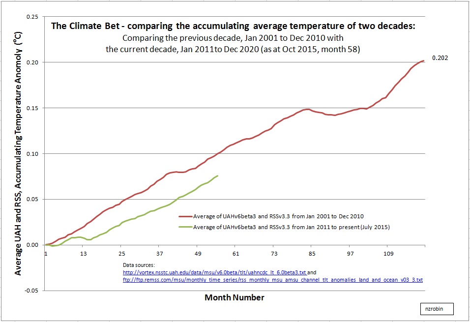
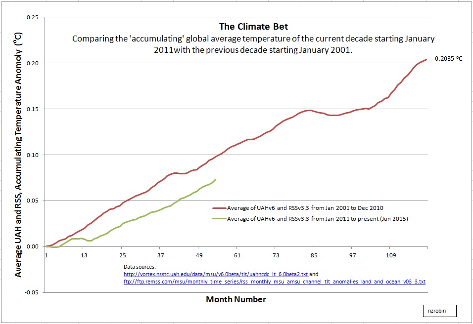
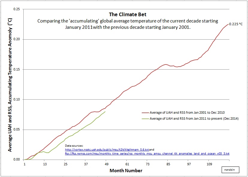
Just in case you were not aware, since about 1997 or so, there has been nearly no global temperature rise. This is despite atmospheric CO2 concentration continuing to rise. To date there are some 55 ideas to explain this slowdown in global warming. Some of the ‘explanations’ presume the so-called ‘greenhouse effect’ is operating as the IPCC models calculated; it’s just that the heat has hidden elsewhere, maybe deep in the ocean.

I wondered if there was empirical data available of the greenhouse effect? And could it show whether or not the greenhouse effect is increasing with increasing CO2, as the IPCC models expect?

First a very quick summary of the IPCC’s greenhouse theory goes something like this.  Increasing CO2 absorbs some of the upwards radiation from the surface, and then re-emits it back toward earth. This has the effect of increasing earth’s atmospheric temperature as outgoing longwave infrared radiation (OLWIR) is reduced by increasing quantities of CO2. Then, recognising that water vapour is the main greenhouse gas, the IPCC models propose that positive feedbacks dominate. This is where some warming leads to increased water vapour, and as water vapour is the main greenhouse gas this increases the greenhouse effect, this further lowers OLWIR, and increases the temperature.

So let’s see how the measurements fit the theory. I needed two data sets, one for OLWIR, and the other global temperature.

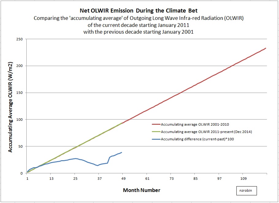
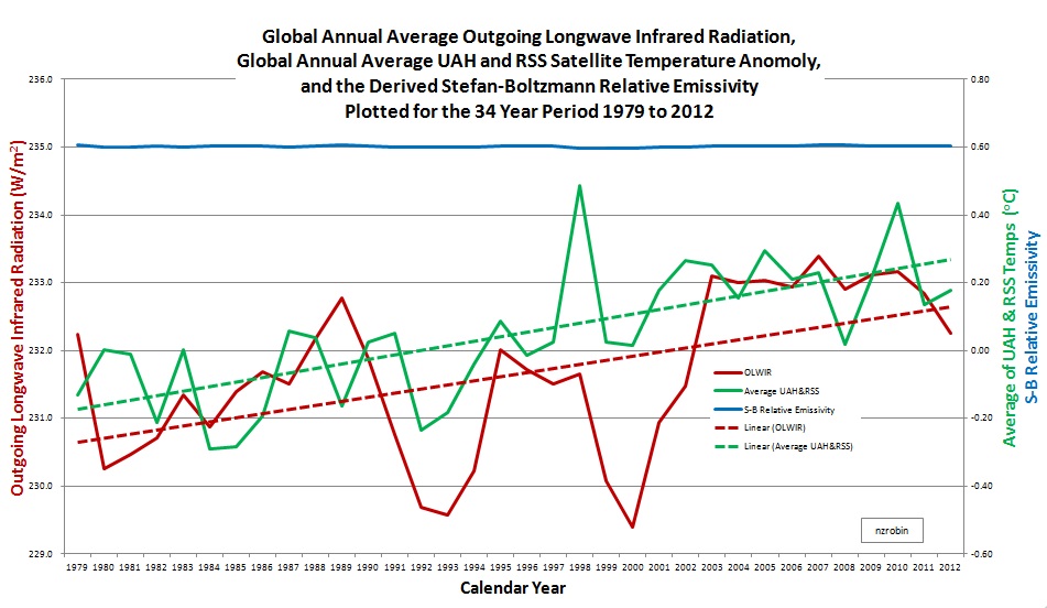
I emailed the National Oceanographic and Atmospheric Administration (NOAA) asking for website directions to their OLWIR data. Their response was quick and I downloaded monthly average OLWIR (W/m2) for each 2.5 degree latitude by 2.5 degree longitude area of the globe. After converting the netCDF files to Excel, I scaled each area’s OLWIR to account for the varying size of the area, resulting in a global average OLWIR. (I used Cosine(Latitude) to approximate the relative areas). (There was also some missing data mid 1994 to early 95. I populated this by a linear interpolation). The resulting annual average OLWIR is shown in the graph below for the years 1979 to 2012. A linear regression fit shows a generally increasing trend in OLWIR over this period.

The temperature data I chose is the average of both University of Alabama Huntsville (UAH) and Remote Sensing Systems (RSS). The result is also plotted on the graph below. A linear regression fit shows a generally increasing trend for years 1979 to 2012. 2013.

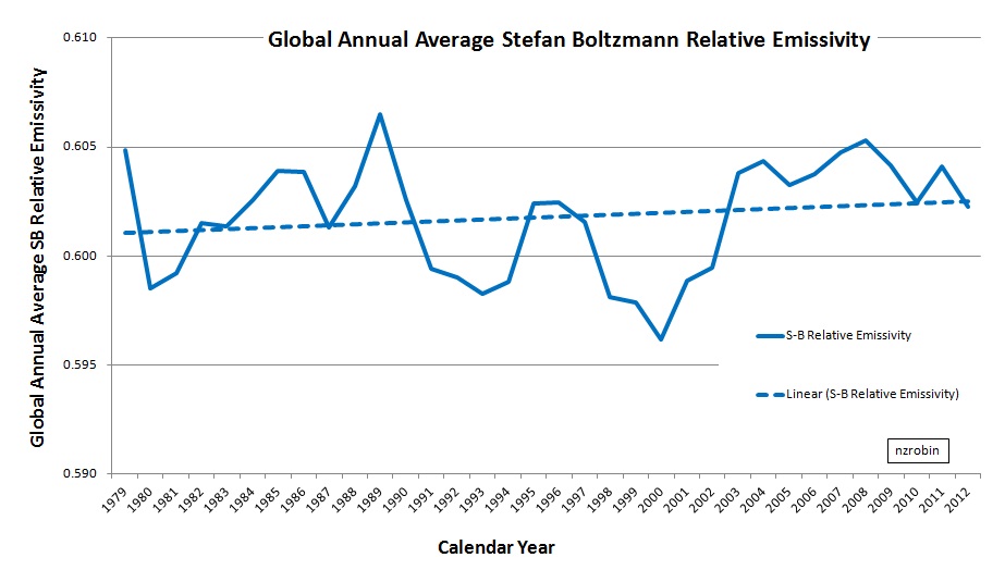
And now we’ll take a look at the Stefan-Boltzmann (SB) relative emissivity trend. Using an average global temperature of 14C, the SB relative emissivity has been derived using E/(K*T^4) for each year and plotted on the graph. If the greenhouse effect was increasing, the relative SB should be declining.  It’s not.  It’s flat lining.

The two primary results of this empirical study are:

The missing heat has gone back to space as it always has – as per SB law, via OLWIR.

And more importantly, the greenhouse effect is not increasing as per IPCC dogma.

There are probably about 55 reasons why … and there’s likely more to be said …

OLWIR, Temp and SB[Additional Material]

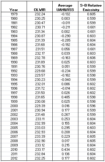
Richard C in his comment below suggested the addition of a graph of the derived relative emissivity at a closer scale. I have added the graph below along with the complete data table used to produce both graphs.

Derived SB data table
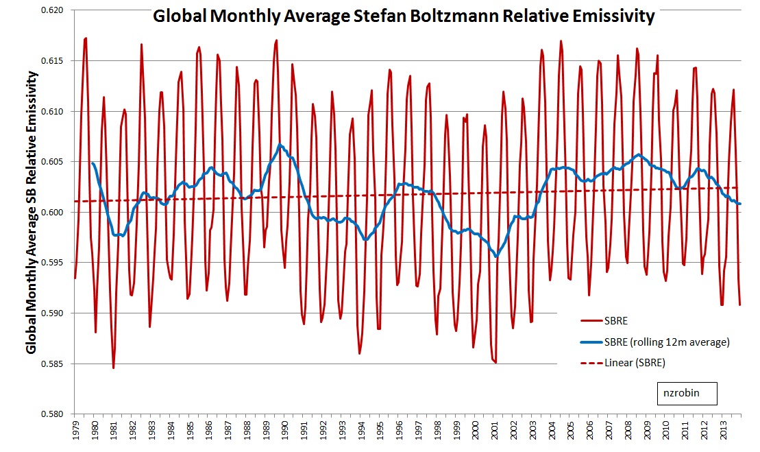
[New material, monthly derived SBRE calculation to compare with annual average calculation, 4 Nov 14]

Monthly SBRE

Link to Data and Graphs.

https://drive.google.com/folderview?id=0BwCJWmtRR6xeeUxlajM5MXVsVXc&usp=sharing
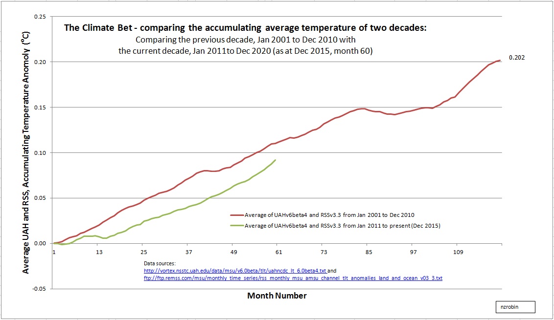


Posted in Climate Science, CO2 | 123 Comments

A Decadal Global Climate Bet – three years down the track

Three years ago, early 2011, a decadal global climate bet was made.  At that time, December 2010 marked the end of a 10 year period.  January 2011 marked the beginning of the next.  The transition stimulated the formation of a decadal global climate bet.  Would the next decade be hotter than the decade just past?  Would it be cooler?  Or would the difference be so little to be statistically insignificant?

And so the coolists (led by Pierre Gosselin – NoTricksZone) and the warmists (led by Rob Honeycutt – Skeptical Science) are having a bet.  They agreed to use a composite of Remote Sensing Systems (RSS) and University of Alabama Huntsville (UAH) lower troposphere temperature – close to the earth’s surface.  The result will be accepted without quibbling, as it was agreed between them that those series are the best that we’ve got.  The average of the two series will decide the bet!

I’ve tried a couple of ways of picturing the comparative ‘race’ between the decades.  The first way is here, and the second way is here.  I prefer the second method, and this is what I have shown below.  It uses an accumulating total, adding 1/120th of the average of the UAH and RSS monthly global anomalies month by month.  The sum of these numbers after 120 months (10 years) is the global decadal average.

Tonight I downloaded the data to December 2013 from UAH and RSS and the graph shows the race position after three complete years.  After three years the coolists are in the lead.

Posted in Climate Science | 6 Comments

A Decadal Global Climate Bet – a second view of the race

About six months ago I posted a short article and a graph attempting to show the progress of a global decadal climate bet.  The graph compared the temperature of the two decades Jan 2001 through Dec 2010 and Jan 2011 to Dec 2020.  I wanted to compare the two decades and make it like a horse race.  To do that, I needed to track progress to date.  Admittedly there’s not much scientific merit in this, but as it is still more than 7 years to the finish line, and that seems like a long time, I thought it might add amusement.

Rob Honeycutt (the leader of the warmist team) kindly visited here a few days ago and left some comments querying the validity of my graph.  They were good comments that got me thinking.  While I reckon the graph is technically correct, it does have some peculiarities which need consideration.  I’ve checked the calculations are correct and they are based on directly downloaded data from UAH and RSS.  The method shows the position between the decades by calculating a running average to date.  Both decades were treated equally and fairly.

But Rob raised a valid point.  The early stages of the graph show a lot of variability, ie: the left side is noisy.  It makes the left side of the graph messy and possibly misleading to some.  The variability is caused by the low number of elements in the sample to date.  As time goes on the noise movement in the average to date diminishes.  And of course, in the end it is the finish line that matters.  The ups and downs only having been interesting along the way.

So thanks Rob, with all that in mind, I have tried another way to look at the race.

The new way does not use an average to date.  It uses instead a simple accumulating counter, adding 1/120th of the average of the UAH and RSS monthly global anomalies to a running total.  The sum of these numbers after 120 months will be the global decadal average.

So take a look at the graph.  Use your eye to extrapolate to the green line to the finish point.  It is still a close race and I’m not game to pick a winner … yet.

Posted in Climate Bet | 6 Comments

Advocating for CO2

Typical newspaper and TV articles which refer to CO2, malign it as a pollutant and some sort of horrible gas that we should do our utmost to get rid of, by not making it, or burying it deep underground.  It is inferred that we’d be far better off without it.

Therefore, as I am able, in any discussion on global warming and the ‘warming’ effect of CO2, I try to frame our perspective of CO2, making reference to the absolutely essential part it plays in the natural life cycles of both plants and animals.  Simply put, without CO2 life would not exist.  It is an essential part of both photosynthesis and respiration.

For instance, on 1 May I was privileged to be able to address a New Plymouth club on global warming.  Early in the presentation, before getting into global warming, I made a few points about the importance of CO2.  Here are the talking point bullets from the slide.

  • CO2 is essential for life
  • Solar energy, CO2 and water, photosynthesis
  • Carbon atom is the building block of life
  • Atmospheric CO2 is where plants get all their carbon
  • Plant growth increases with increased CO2
  • With increased CO2 plants require less water
  • CO2 is not a pollutant, lemonade bubbles, cooking

Recently I was pleased to stumble across a few more instances along these lines.  I recommend them to you.

On 8 May the Wall Street Journal, published an item titled Harrison H. Schmitt and William Happer: In Defense of Carbon Dioxide.

The article starts

“Of all of the world’s chemical compounds, none has a worse reputation than carbon dioxide. Thanks to the single-minded demonization of this natural and essential atmospheric gas by advocates of government control of energy production, the conventional wisdom about carbon dioxide is that it is a dangerous pollutant. That’s simply not the case. Contrary to what some would have us believe, increased carbon dioxide in the atmosphere will benefit the increasing population on the planet by increasing agricultural productivity.”

One of the points made by Schmitt and Happer is that increased CO2 causes increased plant growth.   A week later, on 15 May, a post at The Hockey Schtick highlights a New paper finds a large CO2 fertilization effect greening the globe since 1982.

The abstract of the paper is here  CO2 fertilisation has increased maximum foliage cover across the globe’s warm, arid environments.

“… Using gas exchange theory, we predict that the 14% increase in atmospheric CO2 (1982–2010) led to a 5 to 10% increase in green foliage cover in warm, arid environments. Satellite observations, analysed to remove the effect of variations in rainfall, show that cover across these environments has increased by 11%. Our results confirm that the anticipated CO2 fertilization effect is occurring alongside ongoing anthropogenic perturbations to the carbon cycle and that the fertilisation effect is now a significant land surface process.”

Lubos Motl at The Reference Frame added an interesting perspective with an article titled Why we should work hard to raise the CO2 concentration.

And Andrew Montford at Bishop Hill shared a video of Professor Happer being interviewed by CNBC.

So there you have it.  The most maligned gas in our atmosphere; is essential for life, there is very little of it, and without doubt it ought to be treasured instead.

Posted in Climate Science, CO2, Environment | 3 Comments

The Decadal Global Climate Bet

Just over two years ago, early 2011, a decadal global temperature bet was made.

At that time December 2010 marked the end of the last 10 year period.  January 2011 marked the beginning of the next.  The transition stimulated the formation of a decadal global climate bet.  Would the next decade be hotter than the decade just past?  Would it be cooler?  Or would the difference be so little that the result is statistically insignificant?

And so the warmists and the coolists are having a bet.  It has been agreed to use a composite of Remote Sensing Systems (RSS) and University of Alabama Huntsville (UAH) lower troposphere temperature – close to the earth’s surface. The result will be accepted without quibbling, as it is agreed that it’s the best we’ve got. The average of the two will decide the bet!

The bet started out over at Pierre Gosselin’s site, No Tricks Zone.

http://notrickszone.com/join-the-climate-bet-for-charity/.

So how is it going now that we are now almost a quarter of the way through the race?

Its a close race!  The light blue line shows that the average of Jan 2011 to April 2013 is a whisker cooler than Jan 2001 to April 2003.

(Update note, as at 31 May 2013 the running average is 0.06 deg C cooler)

(Update note, as at 30 June 2013 the running average is 0.051 deg C cooler)


(Note: when I updated the graph with May 2013 data I noticed there was an error with the running average calculation.  This has now been corrected) (Now updated with June 2013 data)

The graph is based on the average of satellite measurements collected and recorded by scientists at the UAH and RSS.  If you want to check the data for yourself, here are the links to the raw data; UAH data and RSS data.


Posted in Climate Science | 16 Comments